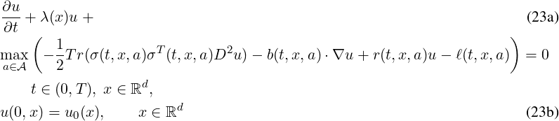
Second order HJB equations and SL scheme

6 Second order HJB equations and SL scheme

The problem solved is the following second order Hamilton-Jacobi (HJ) equation

∂u ∂t-+ λ (x )u + (23a) ( ) max - 1Tr(σ(t,x,a)σT(t,x,a)D2u )- b(t,x,a)⋅∇u + r(t,x,a)u - ℓ(t,x,a ) = 0 a∈A 2 t ∈ (0,T ), x ∈ ℝd, d u(0,x) = u0(x), x ∈ ℝ (23b) \relax \special {t4ht=

where is some non empty compact subset of ℝ^m (m ≥ 1), b(t,x,a) is a vector of ℝ^d, r(t,x,a), ℓ(t,x,a), are real-valued, and σ(t,x,a) is a d × p real matrix (for some p ≥ 1). This problem is linked to the computation of the value function of stochastic optimal control problems.

It is also possible to consider a corresponding steady equation of the form (9a), that is, equation (23a) alone with no term

∂u ---. ∂t \relax \special {t4ht=

It is also possible to consider obstacle equations as for (15), (16) or (17).

The c++ proposed solver is based on an SL method (FD not programmed for this case). ²

Scheme definition: we consider the following SL scheme, implemented on the points x of the grid . The initialization is done by

v0(x) = u0 (x ), x ∈ G. \relax \special {t4ht=

For n = 0,…N_T -1 (time iterations) (or untill some stopping criteria is satisfied in the case of steady equations), for all grid points x ∈, we consider

( ) n+1 e-r(t,x,a)Δt { 1 ∑ ∑ n k,ϵ,u } v (x) := mai∈nA 1-+-λ(x)Δt-( 2p [v ](yx (Δt)) + Δt ℓ(t,x,a )) . (24) 1≤k≤pϵ=±1 \relax \special {t4ht=

where the "characteristics" y_x(h) can be defined, at iteration t = t_n, for some h ≥0, for instance by:

yk,ϵ,a(h) := x + Bk (t,x,a)h + ϵΣk(t,x,a)√h, ϵ ∈ {- 1,1}, k = 1,...,p. (25) x \relax \special {t4ht=

Also, [vⁿ](y) denotes some interpolation of vⁿ at point y (typically Q₁). When using the definition (25), the scheme is of expected order

ϵ O (Δt)+ O (---) Δt \relax \special {t4ht=

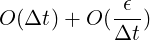
where ϵ is of the order of the interpolation error ∥vⁿ -[vⁿ]∥_∞. For smooth data, this interpolation error is or order Δx² for Q₁ interpolation, where Δx is the spatial mesh size.

An example of data file is given in data/data_SL_order2_2d_diffusion.h.

User inputs:

ORDER=2
PARAMP (denoted p below) This is in general set to p = d in the scheme.
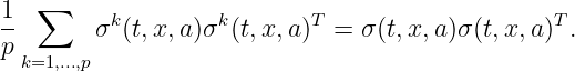
function Sigma: σ(x,k,a,t). A vector of format double[DIM], also denoted σ^k below. This vector should be programmed so as to correspond to the kth column vector of the matrix
$√ -- √-- pσ ≡ ( p σik(t,x, a))i=1,...,d. \relax \special {t4ht=$
More generally, for consistency of the scheme with the PDE, the following relation should hold:
$1 ∑ k k T T p- σ (t,x,a)σ (t,x, a) = σ(t,x,a)σ (t,x,a ) . k=1,...,p \relax \special {t4ht=$
function Drift: b(x,k,a,t), also denoted b^k(t,x,a) below. This is used to define a set of p vectors b^k(t,x,a) (k = 1,…,p) of ℝ^d. For consistency of the scheme with the PDE, the following relation should hold:
$∑ k b (t,x,a) = b(t,x,a). k=1,...,p \relax \special {t4ht=$
For instance the user can set b¹(t,x,a) = B(t,x,a) and b^k = 0, ∀k ≥ 2. One can also set, with p = d: b^k = the k-th component of the b vector, the other components beeing set to zero.
function funcR : r(t,x,a)
function distributed_cost(x,t,x) : distributive cost ℓ(t,x,a).
function discount_factor(x) : λ(x).

[next] [prev] [prev-tail] [front] [up]