3 Model definition header files

The file data/data_simulation.h is the main user’s input file and contains the parameters that define the equation to be solved. It can include an other data_xxx.h file (see basic examples data_basicmodel.h, data_FD_2d_ex1_basic.h).

3.1 Data describing the problem to be solved

The parameter NAME defines the name of the problem that will by used only for shell output during the execution.

State variables and controls .

• DIM: dimension d of the problem

• XMIN[DIM], XMAX[DIM]: the boundary of the computation domain in each direction

• PERIODIC[DIM]: this parameter sets the periodicity for each component of the state variable x:

  • 1 : the variable x_i is periodic

  • 0 : the variable x_i periodic

For a one-player control problem :

• cDIM dimension n_c of the control variable a

• UMIN[cDIM], UMAX[cDIM]: min and max values of the controls in each direction; this defines the set of controls as a cube

  

• NCD[cDIM] number of commands per direction; this defines a grid on the set of controls;

For a two-player control problem :

• cDIM and cDIM2 dimensions n_A and n_B, of the control variables a and b respectively.

• UMIN[cDIM], UMAX[cDIM]: min and max values of the controls a in each direction; this defines the set of controls a in a cube

  

• UMIN2[cDIM2], UMAX2[cDIM2]: min and max values of the controls b in each direction; this defines the set of controls b in a cube

  

• NCD[cDIM] and NCD2[cDIM2] number of controls per direction. This defines a grid for each set of controls.

Dynamics and cost functions For a one-player control problem :

• function dynamics: f(t,x,a) : the dynamics of the controlled system

• function distributed_cost: ℓ(x,a) : the running cost of the optimal control problem

• function discount_factor : λ(x). For steady equations, this function should be strictly positive.

For a two-player control problem :

• function dynamics2: f(t,x,a,b) : the dynamics of the controlled system

• function distributed_cost2: ℓ(x,a,b) : the running cost of the optimal control problem

• function discount_factor : λ(x). For steady equations, this function should be strictly positive.

Special parameters for second order equations

• function funcR : implements the term r(t,x,a) in (6);

• function funcY : implements the term σ(t,x,a) in (6);

Additional computations

• TOPT_TYPE: when an optimal time function associated with the computed solution u is defined this parameter defines what kind of time optimal problem must be solved :

  • TOPT_TYPE=0: the minimum time function is associated with the computed solution u as:

    

    Note that if there is no time t such that u(t,x) ≤ 0, _min(x) is attributed the value INF (a large positive value, defined in stdafx.h, in general set to INF=1e5.

  • TOPT_TYPE=1: the exit time function (hereafter also refered as maximum time function) will be associated with the computed solution u as:

    

    Note that if t exists in [0,T] such that u(t,x) ≤ 0, then _max(x) is attributed a small negative value (i.e., the value -1.e-5).

• COMPUTE_TOPT: should be set to 1 in order that the minimal (resp. maximal) time function be saved in topt.dat, and can be used for optimal trajectory reconstruction when TRAJ_METHOD=0.

• function Vex: if known, the exact solution may be implemented (in that case, set also COMPUTE_VEX=1).

Hamiltonian function and associated parameters

• COMMANDS ∈ {0,1,2}: This parameter indicates how the Hamiltonian function H(x,p) should be defined, using an explicit definition or a definition using a minimization (or a maximization) over a discrete set of controls.

  Case ”COMMANDS=0”: The hamiltonian function H(t,x,p) should be known explicitly. In that case, the user has to define the function Hnum with the expression of a numerical hamiltonian that is consistent with H(x,p). Some examples are given in the file data/data_advancedmodel.h or data_FD_2d_ex1_advanced.h. In addition, the user must complete the function compute_Hconst to define d constants which are bounds for

  

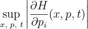
  for each i = 1,…,d (for all x ∈ Ω, all possible gradient values p and times t ∈ [0,T].) This is then used to set the time step Δt in order to satisfy a CFL condition. These constants may also be used in the function Hnum when the Lax-Friedrich numerical hamiltonian is used. (The user may also define directly the constants c_i =Hconst[i] and initialize the previous function accordingly.)

  Case ”COMMANDS=1”: This corresponds to the case when the HJB equation describes the value of an optimal control problem with one player When this value is chosen, the Hamitonian is calculated by optimization over the grid of controls α, as in (3). (Hence the Hamiltonian of the problem may not be explicitly known.) The function Hnum may remain in the header file but will not be used in the computations. Here, the program will use a numerical hamiltonian function corresponding to a finite difference approximation of

  

  as follows:

  

  (here in the case OPTIM=MAXIMUM). Examples can be found in data/data_basicmodel.h (rotation type), or in data/data_FD_2d_ex1_basic.h (eikonal equation).

  Case ”COMMANDS=2”: This corresponds to the case when the HJB equation is related to a two player game, and the Hamiltonian is defined as a min∕max or a max∕min over a set of controls, as in (4a) or (4b). The function Hnum may remain in the header file, but will not be used in the computations. Here, in the case of a max-min Hamiltonian function (i.e., OPTIM=MAXMIN), the following definition of H is used:

  

  The program uses a numerical hamiltonian function corresponding to a finite difference approximation similar to the one-player case, over a set of discretized controls. An example is given in data/data_FD_2d_2c.h

• OPTIM ∈ {MINIMUM, MAXIMUM, MINMAX, MAXMIN}: when COMMANDS=1 or COMMANDS=2, this parameter defines the choice of the optimization type to use in the definition of the Hamiltonian function.

Boundary conditions The parameters are:

• function v0: corresponds to the initial data u₀. This function is also used to initialize the iterations in the case of steady equations.

• BOUNDARY ∈ {0,1,2,3}:

  BOUNDARY=0: means no boundary treatment. The value of v0 will be used in the initialisation to set the boundary (ghost cell) values, and thesel values will remain unchanged afterwards.

  BOUNDARY=1: utilizes Dirichlet boundary conditions for each direction d which is not periodic (i.e., such that PERIODIC[d]=0). The boundary value should be defined in the function g_border.

  BOUNDARY=2: utilizes a mixed boundary condition of the form

  

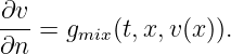
  (where the normal n is pointing outward). Because of the box domain, this corresponds to

  

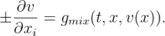
  The function g_bordermix is then used (for each direction d which is not periodic, i.e., such that PERIODIC[d]=0).

  BOUNDARY=3: utilizes a special v_xixi = 0 boundary condition for each direction d which is not periodic (note that this kind of approximation is in general numerically unstable).

  Furthermore, if PERIODIC[d]=1, then periodic boundary conditions will be used in the variable x_d.

• g_border, g_bordermix : used to set different types of boundary conditions.

• BORDERSIZE[dim]: list of integers to define the number of ghost cells used in each direction (at left or right boundary of the domain). For instance, for dim=2, BORDERSIZE[dim]={2,2} defines a boundary with two ghost cells in each direction. In this case, if the mesh size is Nx*Ny, then the grid including ghosts cells is of size (Nx+4)*(Ny+4).

Initial conditions

• EXTERNAL_v0 ∈ {0,1} : If set to 0 (default value), it initializes the first iterate u⁰ for n = 0 with the function v0. Otherwise, if set to 1, then u⁰ is iniatialized by using the values stored in the file OUTPUT/VF.dat (or OUTPUT/VF_PROCxx.dat if parallel MPI is used). This can be used in combination with a prefix EXTERNAL_FILE_PREFIX in order to modify the loaded file (i.e., the prefix of the filename VF.dat).

  EXTERNAL_TOPT ∈ {0,1} : (This parameter is only effective if EXTERNAL_v0=1.) If set to 0 (default value), it initializes the minimal time function as usual. If set to 1, then it will load the previously computed minimal time values from file OUTPUT/topt.dat. This can be used in combination with a prefix EXTERNAL_FILE_PREFIX in order to modify the filename of the loaded file (i.e., the prefix of the filename topt.dat).

  EXTERNAL_FILE_PREFIX (type char) : A prefix that can be used in order to modify the loaded file (i.e., the prefix of the filenames VF.dat and topt.dat). Default value is EXTERNAL_FILE_PREFIX[]=””.

Computation in a subdomain

• COMPUTE_IN_SUBDOMAIN ∈ {0,1}: determines if subdomain computations should be done, so that the evaluation of uⁿ⁺¹(x) is done only at grid mesh points x such that g_domain(x)<0. (For front propagation problems and in the presence of obstacle terms, this can be used in order to reduce significantly the CPU time.)

• function g_domain(x): function used to define the subdomain.

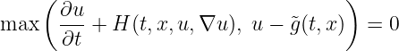
Obstacle terms Instead of solving u_t + H(t,x,u,∇u) = 0, the solver can also treat HJ obstacle equations such as

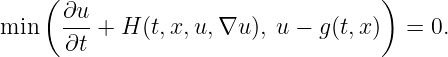
(15)

where g(t,x) is defined by the user. In particular it forces to have u(t,x) ≥ g(t,x) in the case of (15).

Also, the following obstacle equations can be considered:

(16)

or

(17)

where

is user-defined. We will have

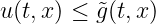
, in the case of (16), or

in the case of (17).

For this, the following parameters are used:

• OBSTACLE ∈ {0,1}

  • 0 : no obstacle g taken into account.

  • 1 : Equation (15) is treated, with the obstacle g .

• function g_obstacle

• OBSTACLE_TILDE ∈ {0,1}

  • 0 : no upper obstacle is taken into account.

  • 1 : Equation (16) is treated, with the upper obstacle function.

• function g_obstacle_tilde

• In the case we set OBSTACLE=1 and OBSTACLE_TILDE=1 then (17) is treated, and both obstacle functions must be defined. The obstacle functions should satisfy

  

  in order to avoid undesired results.

• PRECOMPUTE_OBSTACLE ∈ {0,1}: gives the possibility to precompute all obstacle terms before doing the main iterations. This can reduce CPU time when the obstacle functions are not time-dependent.

3.2 Numerical schemes and associated parameters

Discretization parameters

• ND[DIM] : tab containing the size mesh in each direction (cartesian mesh)

• MESH ∈ {0,1}: default is 1. It utilizes ND[i]+1 points in direction i. (If MESH=0, the mesh points are at the center of the mesh cells, and there are ND[i] points in direction i)

• DT: the time step used for the solver, for the evolutive equation.
  - For the finite difference approach, if DT=0, then time step DT is computed so that the CFL condition be satisfied, that is, such that

  

  where the CFL number belongs to [0, 1]. Otherwise, if DT>0, then the value DT is used for the time step.
  - For the semi-lagrangian approach and for the stationnary equation, the parameter h in the iterative procedure is also set to DT.

Stopping criteria

• T: terminal time

• MAX_ITERATION : to stop the program when this maximum number of iterations is reached.

• EPSILON : for the stopping criteria. If set to 0, do nothing. If set to some positive value ϵ, then the program will stop at iteration n + 1 as soon as

  

  (the L^∞ error between two successive steps is smaller than ϵ).

Therefore, in the case of a time dependent problem, iterations are performed until t_n = T , where the program stops. The parameter EPSILON should be set to 0, and T is used to fix the terminal time. (MAX_ITERATION should be set to a sufficiently large value).

In the case of a steady problem, EPSILON should be set to a strictly positive (small) value, and MAX_ITERATION should be also used to limit the number of maximum iterations in the case of convergence problems. (For debugging purposes, the parameter MAX_ITERATION can also be set to 1 or a small integer value.)

Choice of the solver

• METHOD ∈ {MDF,MSL}:

  MDF: Finite Difference Method. The finite difference method can be used with all possible values of the parameter COMMANDS described before.

  MSL: semi-Lagrangian Method. This method does not use the numerical Hamiltonian function Hnum, rather mainly the dynamics and the distributed costs functions. Important: It is assumed that the Hamiltonian is of the form (3a), (3b). The parameter COMMANDS has no effect on the method. (The case of max-min or min-max, i.e. (4a) or (4b) is not yet supported by the software.)

3.2.1 Finite Difference Method

This method is used when METHOD=MDF. The user has to set the following scheme discretization parameters:

• CFL ∈]0, 1[: the constant of the CFL condition that is used in finite difference methods to adjust the time step DT.

• TYPE_SCHEME ∈ {LF,ENO2}: type of spacial discretization

  • LF: Lax-Friedrich scheme (first order scheme)

  • ENO2 : ENO scheme of second order to approximate the derivatives ∇u

• TYPE_RK ∈ {RK1,RK2,RK3}: time discretization by a Runge-Kutta method of order 1, 2 or 3.

  • RK1 : RK method of order 1

  • RK2 : RK method of order 2

  • RK3 : RK method of order 3

3.2.2 Semi-Lagrangian Method

This method is used when METHOD=MSL. One needs to define :

• TYPE_SCHEME ∈ {STA,EVO}:

  • STA : stationnary case, for solving (7a). In this case, the scheme is based on an iterative procedure.

  • EVO : dynamic case (should be default value) for solving (1). It is also advised to use this mode to solve steady equations, and a stopping criteria based on the parameter EPSILON.

• ORDER ∈ {1,2}: this value is set to 1 for solving first order equations and to 2 to solve second order equations (see other section below for second order HJB equations).

• TYPE_STA_LOOP ∈ {NORMAL,SPECIAL}: Mesh loop order during mainloop for the stationary case

  • NORMAL : normal ordering loop

  • SPECIAL: special ordering loop (makes 2^d loops at each iteation, modifiying the current values of the value v during each loop)

• TYPE_RK ∈ {RK1_EULER,RK2_HEUN,RK2_PM}:

  • RK1_EULER : RK1 Euler scheme

  • RK2_HEUN : RK2 Heun scheme

  • RK2_PM : RK2 Mid-point scheme

• INTERPOLATION ∈ {BILINEAR,PRECOMPBL,DIRPERDIR}:

  • BILINEAR : (default value) bilinear interpolation (Q1 interpolation)

  • PRECOMPBL : precompute the interpolation coefficients (to use with tiny mesh sizes)

  • DIRPERDIR : another interpolation method (obsolete)

• P_INTERMEDIATE : number of intermediate time steps to go from t_n to t_n + Δt for computing a characteristic for a given RK method.

3.3 Value problems defined implicitly

Some special computations can be made in addition to solving the HJB equation in the case when the computed d-dimensional solution function u is used to characterize the epigraph of an other value function v of a d - 1 dimensional problem. This approach is used for general state-constrained value problems as described in [1], where the problem is set back to a state-constrained reachability problem. It is assumed that both value functions are related to each other as follows:

(18)

So the value function v can be considered as being implicitly defined by the computed function u.

• VALUE_PB ∈ {0,1}: to allow these additional computations, set VALUE_PB=1.

Also when VALUE_PB=1 it is assumed that only the last state variable, x_d, can be used to define an implicit value function. This convention must be taken into account when defining the dynamical system and its parameters in the header file.

3.4 Execution and output parameters

The main purpose of the library is to solve the HJB - type equations. In addition, it is possible to compute and save some associated functions during the main computation. It is also possible to work with optimal trajectory algorithms, after the computation of the solution. The main computation to solve the PDE is most time and memory consuming part of the work. Once the solution computed and saved one can run the program many times to compute different trajectories from this data without need to make the main loop computation at each time. To choose the execution modes the user can use the following parameters (see below).

All the output files generated during an execution are generaly saved in the folder OUTPUT/ (the user may use other names for the output files and output directory, see file include/stdafx.h (or src/stdafx.h) although it is recommanded to not modify the filenames).

• COMPUTE_MAIN_LOOP:

  • 1 : the main computational loop (iterative scheme) is called

  • 0 : the main loop is not called, only data initializations, trajectory computations and savings are performed. This is useful if a previous HJB computation has been made and that only new trajectories have to be computed. There is no need to recompute the value function or the minimal time function. The program will then load the needed values (value function and/or minimal time function) in order to perform trajectory reconstructions, or to perform particular savings.

• COMPUTE_VEX ∈ {0,1}: will save the exact solution on the grid in a file.

  • 1 : the solution programmed in the user function Vex will be saved.

  • 0 : no saving.

  In particular it allows to ocompute errors (see below) relatively to the value of Vex.

• COMPUTE_TOPT ∈ {0,1}: will compute an optimal time function associated with the solution u. Recall that the type of optimal time function is defined by the parameter TOPT_TYPE (see (13) and (14)). The computed function will be saved at the end of the computation.

• PRECOMPUTE_COORD:

  • 1 : precomputes the coordinates: faster computations but more memory demanding.

  • 0 : no precomputations.

• CHECK_ERROR ∈ {0,1}: is set to 1 then computes the error every CHECK_ERROR_STEP steps (L^∞ and L¹ error computations) Errors are relative to the Vex function. Furthermore, the parameter C_THRESHOLD defines the region where the errors will be computed : the region of points x such that

  

3.5 Parameters for trajectory reconstruction

The dynamics used for the trajectory reconstruction algorithms is the one defined in the function dynamics (in the case COMMANDS=0 or 1) or dynamics2 (in the case COMMANDS=2). Related reconstruction procedures are located, if available, in the files

src/compute_ot.h (reconstruction based on an optimal time function)
src/compute_otval.h (reconstruction based on the value function)
src/find_oc.h

For two-player games, the reconstruction procedure is programmed in

src/compute_ot2.h (reconstruction based on an optimal time function)
src/find_oc2.h.

The following parameters are used:

• TRAJPT ∈ {0,1,...}: set to 1 or greater for trajectory reconstruction, 0 otherwise. When TRAJPT=N, with N ≥ 1 this defines the number of trajectories to compute for N initial conditions.

• initialpoint[TRAJPT*DIM]: the set of coordinates of all initial points (put the list of all the TRAJPT*DIM coordinates, one point after another, if there is more than one initial point).

• TRAJ_METHOD ∈ {0,1} : this is two methods of trajectory reconstruction.

  0: based on the minimal time (if TOPT_TYPE=0), or exit time (if TOPT_TYPE=1)

  1: based on the value function (utilizes the VFxx.dat files).

  Furthermore, if COMMANDS=1, then the function dynamics is used for the dynamics (one control). If COMMANDS=2, the function dynamics2 is used (two controls).

• time_TRAJ_START: starting time t₀ used in the case TRAJ_METHOD=1. The value t₀ may belong to [0,T[ or be such that t₀ < 0.

  In the case t₀ ∈ [0,T[: The program will construct an approximated trajectory such that ẏ(t) = f(t,y(t),α(t)), t ∈ [t₀,T], and starting with y(t₀) = x₀ as initial point. More precisely, if v(t_n,x) is the value function at time t_n, the procedure aims at constructing a control a = aⁿ (and associated trajectory y _tn,x^a(t _n+1)) that realizes a minimum in

  

  is minimal (resp. maximal) in the case OPTIM=MAXIMUM (resp. the case OPTIM=MINIMUM).

  In the case t₀ < 0: the program will look for a first value t_n (n = 0,…,N - 1) such that v(t_n,x) > 0 and v(t_n+1,x) < 0, and will then reconstruct a trajectory with starting time t = t_n (if v(t₀,x) < 0 then the trajectory will start from t = t₀).

• If TRAPJT=0 then one should define accordingly initialpoint[0]={}.

Now we describe some stopping criteria which are used in the trajectory reconstruction routines.

• g_target: a user-defined function, such that g_target(x)<=0 if x belongs to a "target" set.

• TARGET_STOP ∈ {0,1}: default is 0. If we set TARGET_STOP=1, then the program will furthermore stop the trajectory reconstruction when

  

  and will declare this as a successfull trajectory reconstruction (success=1 in the output file successTrajectory.dat). This option can be useful when the trajectory reconstruction is based on the value function (TRAJ_METHOD=1) and that we want to furthermore stop the trajectory reconstruction when a given region is reached.

• min_TRAJ_STOP (double): The trajectory reconstruction is stopped when

  

  and declare this as a successfull trajectory reconstruction (success=1 in the output file successTrajectory.dat). Notice that in the case when TRAJ_METHOD is 0, linked to optimal time reconstruction procedures, the value val(x) corresponds to the value of topt(x) at point x; in the case when TRAJ_METHOD=1, val(x) corresponds to the value function at the given time of reconstruction and at point x.

  In general the minimal time is zero on a target set, and it can be numerically difficult to reach exactly topt(x)=0. So this parameter can be set to a small non zero value to allow some margin error to stop the trajectory reconstruction.

• max_TRAJ_STOP (double): The trajectory reconstruction is also stopped when

  

  and will declare this as an unsuccesfull trajectory reconstruction (success=0 in the output file successTrajectory.dat). This can be used to detect when val(x)=INF or some large value, showing that we enter a forbidden region and that the trajectory reconstruction should be stopped.

In the case COMMANDS=2 (in the presence of an adverse control denoted u2), it is possible to reconstruct trajectories by setting TRAJ_METHOD=0 (using the minimal time function approach) and using the following; the function dynamics2 is used to describe the dynamics for the two-control case.

• ADVERSE_CONTROL∈{0,1}: default value is 0. It will then find the best strategy of controls u for the worst case situation on the adverse control u2. If ADVERSE_CONTROL=1, then it will use the adverse control u2 as defined by the function u2_adverse.

• u2_adverse(t,x,u2): user-defined function, to define in u2 an adverse control depending on time t and position x.

The following can be used for more outputs concerning trajectory reconstructions:

• PRINT_TRAJ ∈ {0,1} : default is 0. If set to 1, more outputs on trajectory reconstruction are given in the current window.

3.6 Output parameters and files

Output files are generally contained in the directory OUTPUT/. (It is possible to use other names for the output files and output directory, see file include/stdafx.h, although it is recommanded not to do so.)

3.6.1 Savings options

• FILE_PREFIX (type char) : This character string will be prefixed to all filenames that will be saved during the execution. The default value is an empty char: char FILE_PREFIX[]=””. In this case the default file names will be used. Notice that each new execution of the program will erase all previously generated data having the same file name. Hence one way to keep precomputed datas is to use the prefix FILE_PREFIX parameter in order to add it to the output filenames. (In the same way, EXTERNAL_FILE_PREFIX can be used to change the name of some loaded data files for starting computations in particular cases. See EXTERNAL_v0)

• SAVE_VF_ALL ∈ {0,1}: to save the value of u each SAVE_VF_ALL_STEP iterations. The default names of generated files are OUTPUT/VFn.dat where n is the number of file.

  SAVE_VF_ALL_STEP (≥ 1).

• SAVE_VF_FINAL ∈ {0,1}: to save the value of u at the last iteration. The default name of the generated file is OUTPUT/VF.dat. (Set to 1 in particular if recomputations with different COUPE parameters - see below - is used, while the value is not recomputed - COMPUTE_MAIN_LOOP=0)

• SAVE_VF_FINAL_ONSET ∈ {0,1}. Set to 1 to save the interpolated values of the final value function u on a given, user-defined set of points. The data must be defined in OUTPUT/X_user.dat (default name): each line of this file must contain the d coordinates of a point for which one want to compute and save the value function. The generated file is OUTPUT/XV_user.dat (default name).

• SAVE_VALUE_ALL ∈ {0,1}. Assumes VALUE_PB=1. Set to 1 to save the implicit value v at each SAVE_VALUE_ALL_STEP iteration. The default names of generated files are OUTPUT/VALUE_n.dat where n is the number of file.

• SAVE_VALUE_FINAL ∈ {0,1}. Assumes VALUE_PB=1. Set to 1 to save the value of the implicit value function v at the last iteration. The default name of the generated file is OUTPUT/VALUE.dat.

• The file OUTPUT/VEX.dat is saved if COMPUTE_VEX=1. It contains the final exact solution value as programmed in Vex.

• COUPE_DIMS[DIM], COUPE_VALS[DIM]:
  - list of integers n_i (0 or 1) to define the two variables used for the cut.
  - list of values (c_i or 0.) to define the position of the cut. The values c_i are used only when n_i = 0.

  These parameters allows to save some lower-dimensional slice of the output files:
  - A file OUTPUT/coupe.dat is saved (corresponding to a slice of VF.dat).
  - A file OUTPUT/coupeex.dat is also saved in the case COMPUTE_Vex=1.
  - A file OUTPUT/toptcoupe.dat is also saved in the case COMPUTE_TOPT=1.
  Example : COUPE_DIMS[DIM]={1,0,1} and COUPE_VALS[DIM]={0.,0.5,0.} (in the case DIM=3) defines a slice in the plane x₂ = 0.5.

3.6.2 Data formatting options

• FORMAT_FULLDATA ∈ {0,1}: defines the format of the data files for value functions savings (such as VF.dat, ...). This parameter does not affect files such as coupe.dat

  • FORMAT_FULLDATA=1: The file is structured as follows, on each line

    

    where val corresponds to the value u(T,x) at mesh point x = (x_i1,…,x_id).

  • FORMAT_FULLDATA=0: each line, in the same order, contains the value

    

3.6.3 General data files

• OUTPUT/filePrefix.dat. This file contains the value of FILE_PREFIX[] parameter. It is used also by the visualization routines to retrieve all the other files generated for a given model.

  Important remark. The name of this file does not change if a non empty FILE_PREFIX[] is defined. This is the unique file that has always the same name. All the other files are given here with their default names, but are named with the user’s prefix as follows:

  

• OUTPUT/data.dat (default name): This file is saved when the main loop computation is finished. It contains the most important parameters values for the solved problem : the dimension of the state variable and controls, the computational domain, the number of grid points in each direction. Theses data are essential to retrieve the real values of space variables from their integer indexes saved in the formatted value files. This file is used in particular by the plotting functions for matlab/octave given with the library (see the section below).

• OUTPUT/Dt.dat (default name): This file contains the value of the time step used for the solution iterations. This value is used by the trajectory reconstruction algorithms.

3.6.4 Files related to trajectory reconstruction

• OUTPUT/traj-n.dat: If TRAJPT≥ 1, the file corresponds to the trajectory number n. Each line has the form

  

  where xi are the coordinates of the point at time t, and aj the corresponding control parameters. Adverse controls bj may also be present, as follows:

  

• OUTPUT/successTrajectories.dat: Each line n of this file has the form

  

  and indicates whether the trajectory number n was successful or not (success=1 or 0) and shows the corresponding terminal coordinates (xi) and time t of the last constructed point.

3.7 Advanced parameters

• function init_data(): it is empty by default. It is called when the execution starts, before the initialization of all HJB objects. The user can complete this function if necessary to initialize some model specific parameters. This can be useful for some complex applications.

• function post_data(): this function is empty by default. It is called at the end of the execution, after all standard HJB computations. The user can complete this function if necessary to define some model specific data transformations. This can be useful for some complex applications.